Notes on Algorithmic Game Theory

Notes on Algorithmic Game Theory based on lecture notes by Prof. Tim Roughgarden. Originally written along with Mustansir Mama for a study project, done under the guidance of Prof. Abhishek Mishra.

Introduction: Mechanism Design

The field of Mechanism Design studies the science of rule making. The goal of the field is to design rules so that strategic behaviour by participants lead to a desirable outcome. Mechanism Design finds applications in Internet search auctions, wireless spectrum auctions etc.

##The Price Of Anarchy

The Price of Anarchy (POA) is defined to be the ratio of the system’s performance with strategic participants to the best possible system performance.

Braess’s Paradox

Braess’s Paradox is an example of a situation where selfish behaviour is not essentially benign. Consider two cities $s$ and $t$ connected by two routes, one through $v$ and the other through $w$. Each route comprises of one long wide road with a constant travel time of one hour and one short narrow road with travel time in hours equal to the fraction of traffic using it (refer Figure 1(a)). The total travel time in hours of the two edges on one of these routes is $1 + x$, where $x$ is the fraction of the traffic that uses the route. The two routes are hence identical and, at equilibrium, traffic should be equal in both. In this case, all drivers arrive at $t$ an hour and a half after leaving $s$.

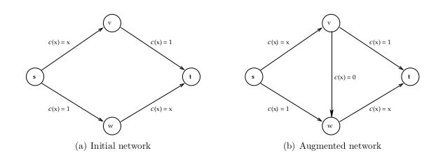Figure 1: Braess’s Paradox

Now, suppose we install a teleporter which lets drivers travel instantly from $v$ to $w$. The new network is shown in Figure 1(b), with the teleporter represented by edge $(v, w)$ with constant cost $c(x) = 0$, independent of the traffic on the road. With this added edge, the traffic pattern in the network will change. The travel time along the new route $s \rightarrow v \rightarrow w \rightarrow t$ is never worse than that along the two original paths, and it is strictly less whenever some traffic fails to use it. We therefore expect all drivers to switch to the new route. Because of the resulting traffic on the edges $(s, v)$ and $(w, t)$, all of these drivers now experience two hours of travel time when driving from $s$ to $t$.

Braess’s Paradox shows that selfish routing does not minimize the commute time of the drivers — in the network with the teleportation device, an altruistic dictator could dictate routes to traffic in improve everyone’s commute time by 25%. For the network in Figure 1(b),

\[\begin{aligned} \text{the price of anarchy (POA)} &= \frac{2}{\frac{3}{2}}\\ &= \frac{4}{3}. \end{aligned}\]

Complexity of Equilibria

Informally, an equilibrium is a “steady state” of a system where each participant, assuming everything else stays the same, wants to remain unchanged. In most games, the best move to take depends on what the other participants are doing. Rock-Paper-Scissors, rendered below in “bimatrix” form, is an established example.

	Rock	Paper	Scissors
Rock	0, 0	-1, 1	1, -1
Paper	1, -1	0, 0	-1, 1
Scissors	-1, 1	1, -1	0, 0

One player chooses a row and the other a column. The numbers in the corresponding matrix entry are the payoffs for the row and column player, respectively. There is certainly no “deterministic equilibrium” in the Rock-Paper-Scissors game: whatever the current state, at least one player would benefit from a unilateral move.

A crucial idea is to allow randomized strategies. If both players randomize uniformly in Rock-Paper-Scissors, then neither player can increase their expected payoff via a unilateral deviation. Every unilateral deviation yields zero expected payoff to the player deviating. A pair of probability distributions with this property is a mixed-strategy Nash equilibrium. Remarkably, with randomization, every game has at least one Nash equilibrium.

Nash’s Theorem

Nash’s Theorem: Every game with a finite number of players has a Nash equilibrium.

Furthermore, if a bimatrix game is zero-sum, that is, the payoff pair in each entry sums to zero, then the Nash equilibrium can be computed in polynomial time. This can be done via linear programming or, if a small amount of error can be tolerated, via simple iterative learning algorithms.

Under suitable complexity assumptions, there is no polynomial-time for computing a Nash equilibrium in general (non-zero-sum) games. While the problem is not NP-hard (unless $NP = coNP$), it is PPAD-hard, that is, of intermediate hardness like graph isomorphisms and factoring problems, and is unlikely to be in P or NP-complete.

Single Item Auctions

In a single item auction, there is some number $n$ of strategic participants (bidders) who are interested in buying the item. Each bidder $i$ has a valuation $v_{i}$ which is its maximum willingness to pay for the item being sold. Thus bidder $i$ wants to acquire the item as cheaply as possible, provided that the selling price is at most $v_{i}$. This valuation is private, meaning that it is unknown to other bidders and the seller.

The utility model, known as the quasi-linear utility model is as follows.

\[\text{utility } \textit{u}= \begin{cases} 0,& \text{if bidder } \textit{i} \text{ loses}\\ {v_{i} - p},&\text{if bidder } \textit{i} \text{ wins at a price } \textit{p}\\ \end{cases}\]

Sealed-Bid Auctions

In a sealed-bid auction,

1. Each bidder $i$ privately communicates a bid $b_{i}$ to the auctioneer in a sealed envelope.
2. The auctioneer decides who gets the good (if anyone).
3. The auctioneer decides the selling price.

First-Price Auctions

In a first-price auction, the highest bidder wins and is asked to pay its bid.

First-price auctions are hard to reason about. First, as a participant, it’s hard to figure out how to bid. Second, as a seller or auction designer, it’s hard to predict what will happen. A bidder would have to pick his bid such that it is higher than the bids of other participants, but still small enough to get a considerable utility gain.

Second-Price Auctions

In a second-price or Vickrey auction, the highest bidder wins and pays an amount equal to the second-highest bid. In a Vickrey auction, every bidder has a dominant strategy: set its bid $b_{i}$ equal to its private valuation $v_{i}$. This strategy maximizes the utlity of bidder $i$ no matter what other bidders do.

This means that second-price auctions are particularly easy to participate in. One does not need to reason about other participants. One’s bid only depends on one’s private valuation and nothing else. Also, in a Vickrey auction, every truthtelling bidder is guaranteed non-negative utility.

Awesome Auctions

An awesome auction is one with the following properties:

1. [Strong incentive guarantees] It is dominant-strategy incentive-compatible (DSIC), i.e., every bidder has a dominant strategy (to bid its private valuation) and truthful bidding guarantees non-negative utility.
2. [Strong performance guarantees] If bidders report truthfully, then the auction maximizes the social surplus \(\sum_{i=1}^{n} v_i x_i\).
3. [Computational efficiency] The auction can be implemented in polynomial time.

Sponsored Search Auctions

A Web search results page comprises a list of organic search results deemed by some underlying algorithm to be relevant to you query along with a list of sponsored links, which have been paid for by advertisers.

The goods for sale are the $k$ slots for sponsored links on a search results page. The bidders are the advertisers who have a standing bid on the keyword that was searched on. Such auctions are more complex than single-item auctions in two ways. First, there are generally multiple goods for sale (i.e., $k > 1$). Second, these goods are not identical — slots higher on the search page are more valuable than lower ones, since people generally scan the page from top to bottom.

The click-through rate (CTR), $\alpha_j$, of a slot represents the probability that the end-user clicks on the slot. Ordering the slots from top to bottom, we make the reasonable assumption that $\alpha_1 \geq \alpha_2 \geq … \geq \alpha_k$. We assume that an advertiser is not interested in an impression (i.e., being displayed on a page), but rather has a private valuation $v_i$ for each click on its link. Hence, the value derived by advertiser $i$ from slot $j$ is $v_i \alpha_j$.

Designing A Sponsored Search Auction

While creating an auction system, we need to design two things at once, the choice of who wins what (allocation rule), and the choice of who pays what (payment rule). In many applications including sponsored search auctions, we can tackle this two-prong design problem one step at a time.

Step 1: Assume, without justification, that bidders bid truthfully. Then, how should we assign bidders to slots so that properties (2) and (3) of awesome auctions hold?

Step 2: Given our answer to Step 1, how should we set selling prices so that property (1) of awesome auctions holds?

Step 2 ensures the DSIC property which means that bidders will bid truthfully. This satisfies the hypothesis in Step 1, and so, the final outcome of the auction is indeed surplus-maximizing and can be computed in polynomial time.

For Step 1, we assign the $j^{th}$ highest bidder to the $j^{th}$ highest slot for $j = 1, 2, \dots, k$. Step 2 can be solved using Myerson’s Lemma, a powerful tool in mechanism design.

Myerson’s Lemma

Single-Parameter Environments

A single-parameter environment has some number $n$ of bidders, each with some private valuation $v_i$, and a feasible set $X$. Each element of $X$ is an $n$-vector $(x_1,x_2,\dots,x_n)$ where $x_i$ denotes the amount of stuff given to bidder $i$. For instance:

1. In a single-item auction, $X$ is the set of 0-1 vectors that have at most one 1, i.e. $\sum_{i=1}^{n} x_i \leq 1$.
2. If there are $k$ identical goods and each bidder gets at most one, $x$ is the set of 0-1 vectors satisfying the condition $\sum_{i=1}^{n} x_i \leq k$.
3. In sponsored search auctions, $X$ is the set of $n$-vectors, such that if bidder $i$ is assigned to slot $j$, then the component $x_i$ equals the CTR $\alpha_j$ of its slot.

Allocation and Payment Rules

A sealed-bid auction has three steps:

1. Collect bids $\mathbf{b} = (b_1, b_2,\dots,b_n)$
2. [Allocation rule] Choose a feasible allocation $x(b) \in R^n$ as a function of the bids.
3. [Payment rule] Choose payments $p(b) \in R^n$ as a function of the bids.

According to the quasi-linear utility model, bidder $i$ has utility,

\[u_i(\mathbf{b}) = v_i \cdot x_i(\mathbf{b}) - p_i(\mathbf{b})\]

Implementable and Monotone Allocation Rules

An allocation rule $x$ for a single-parameter environment is implementable if there is a payment rule $p$ such the sealed-bid auction $(x, p)$ is DSIC.

An allocation rule $x$ for a single-parameter environment is monotone if for every bidder $i$ and bids \(\mathbf{b}_{-i}\) by the other bidders, the allocation \(x_i(z,\mathbf{b}_{-i})\) to $i$ is non-decreasing in its bid $z$.

Myerson’s Lemma

Myerson’s Lemma^[8]: Fix a single-parameter environment.

1. An allocation rule $x$ is implementable if and only if it is monotone.
2. If $x$ is monotone, then there is a unique payment rule such that the sealed-bid auction $(x,p)$ is DSIC.
3. The payment rule in (b) is given by an explicit formula,

\[p_i(b_i,\textbf{b}_{-i}) = \int_0^{b_i}z \cdot \frac{d}{dz}x_i(z,\textbf{b}_{-i})dz \tag{1}\]

For constructing DSIC mechanisms, we require an implementable allocation rule. However, there is no obvious and straighforward way to check if an allocation rule is implementable. Part (a) of Myerson’s Lemma provides an equivalence between the definitions for implementable and monotone allocation rules. In most cases, it is not difficult to check if an allocation rule is monotone. This equivalence hence helps us find implementable allocation rules. Part (b) of the lemma assures that there is no ambiguity as to how to assign a payment rule to an implementable allocation rule. For each implementable allocation, there is a unique payment rule which makes it DSIC. This payment rule is given explicitly by the formula in Part (c).

Applying Myerson’s Lemma to Sponsored Search Auctions

Our allocation rule assigns the $j^{th}$ highest bidder to the $j^{th}$ highest slot for $j = 1, 2, \dots, k$. Consider a bid vector $\mathbf{b}$ reindexed such that $b_1 \geq b_2 \geq \dots \geq b_n$. Consider the first bidder and imagine increasing its bid from 0 to $b_1$ , holding the other bids fixed. The allocation \(x_i(z, \mathbf{b}_{-i})\) ranges from 0 to $\alpha_1$ as $z$ ranges from 0 to $b_1$, with a jump of $\alpha_j - \alpha_{j+1}$ at the point where $z$ becomes the $j^{th}$ highest bid in the profile, namely $b_{j+1}$. Thus, in general, Myerson’s payment formula specializes to

\[p_i(\mathbf{b}) = \sum_{j=i}^k b_{j+1}(\alpha_{j} - \alpha_{j+1}) \tag{2}\]

for the $i^{th}$ highest bidder (where $\alpha_{k+1} = 0)$.

Therefore, the per-click payment for bidder (or slot) $i$ is simply (2) scaled by $\frac{1}{\alpha_i}$:

\[p_{i}(\mathbf{b}) = \sum_{j=i}^k b_{j+1}\frac{\alpha_{j} - \alpha_{j+1}}{\alpha_{i}} \tag{3}\]

Knapsack Auctions

In a knapsack auction,

1. Each bidder $i$ has a publicly known size $w_i$ (the duration of a TV ad, the size of files it wants to store on a shared server etc.).
2. Each bidder has a private valuation $v_i$ (the bidder’s willingness-to-pay for its ad being shown on TV, or to have its data hosted on the shared server).
3. The seller has a capacity $W$ (the length of a TV commercial break or the size of a shared server).

A Surplus-Maximizing DSIC Mechanism

For a knapsack auction to be an awesome auction, it must maximize social surplus. Hence, its allocation rule is given by

\[\mathbf{x(b)} = \underset{X}{\operatorname{arg max}} \sum_{i=1}^n b_ix_i \tag{4}\]

That is, the allocation rule solves an instance of the Knapsack problem in which the item values are given by the bids $b_1,\dots,b_n$, and item sizes are the a priori known sizes $w_1,\dots,w_n$. By definition, if bidders bid truthfully, this allocation maximizes social surplus.

Critical Bids

Myerson’s Lemma (parts (a) and (b)) guarantees the existence of a payment rule p such that the mechanism \((\mathbf{x}, \mathbf{p})\) is DSIC. This payment rule is easy to understand. Fix a bidder $i$ and bids \(\mathbf{b}_{-i}\) by the other bidders. Since the allocation rule is monotone and $0-1$, the allocation curve \(x_i (·,\mathbf{b}_{-i})\) is extremely simple: it is $0$ until some breakpoint $z$, at which point it jumps to $1$ (Figure 1).

Thus, if $i$ bids less than $z$, it loses and pays 0. If $i$ bids more than $z$, it pays $z\cdot(1-0) = z$. That is, $i$ pays its critical bid — the lowest bid it could make and continue to win (holding the other bids $\mathbf{b}_{-i}$ fixed).

Intractability of Surplus Maximization

The mechanism detailed above is not an awesome auction. The reason is that the Knapsack problem is NP-hard. Thus there is no polynomial-time implementation of the allocation rule unless $P = NP$. Hence, properties (2) and (3) of awesome auctions are incompatible for knapsack auctions.

This fact motivates us to relax at least one of the three goals of awesome auctions. Relaxing property (1) will not help at all since it is the other two properties that conflict. As the knapsack problem can be solved in $O(nW)$ (pseudopolynomial) time, relaxing (3) is a perfectly valid move.

Algorithmic Mechanism Design

Algorithmic mechanism design is one of the initial and most well-studied branches of algorithmic game theory. The dominant paradigm in algorithmic mechanism design is to relax the second constraint (optimal surplus) as little as possible, subject to the first (DSIC) and third (polynomial-time) constraints.

Algorithmic mechanism design bears a strong similarity to the field of approximation algorithms. The primary goal in approximation algorithms is to design algorithms for NP-hard problems that are as close to optimal as possible subject to a polynomial-time constraint. Algorithmic mechanism design has exactly the same goal, except for an additional monotonicity constraint.

Near-Surplus-Maximizing Polynomial-Time Knapsack Auctions

The following greedy algorithm is a $\frac{1}{2}$-approximation algorithm for the Knapsack problem.

1. Sort and re-index the bidders so that \(\frac{b_1}{w_1} \geq \frac{b_2}{w_2} \geq \dots \geq \frac{b_n}{w_n}\)
2. Pick winners in this order until one doesn’t fit, and then halt.
3. Return either the step (2) solution, or the highest bidder, whichever creates more surplus.

The Revelation Principle

Revelation Principle: For every mechanism M in which every participant has a dominant strategy (no matter what its private information), there is an equivalent direct-revelation DSIC mechanism $M’$.

By assumption, for every participant $i$ and private information $v_i$ that $i$ might have, $i$ has a dominant strategy $s_i(v_i)$ in the given mechanism $M$. We construct the following mechanism $M’$, to which participants delegate the responsibility of playing the appropriate dominant strategy.

1. Direct-revelation mechanism $M’$ accepts sealed bids $b_1,\dots,b_n$ from the players.
2. It submits the bids $s_1(b_1),\dots,s_n(v_n)$ to the mechanism $M$, and chooses the same outcome (e.g., winners of an auction and selling prices) that M does.

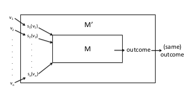Figure 2: Proof of the Revelation Principle.

Revenue-Maximizing Auctions

Bayesian Analysis

The average-case or Bayesian analysis model consists of:

• A single-parameter environment.
• The private valuation $v_i$ of participant $i$ is assumed to be drawn from a distribution $F_i$ with density function $f_i$ with support contained in $[0, v_max ]$. We assume that the distributions $F_1, \dots ,F_n$ are independent (but not necessarily identical). In practice, these distributions are typically derived from data, such as bids in past auctions.
• The distributions $F_1, \dots ,F_n$ are known in advance to the mechanism designer. The realizations $v_1,\dots,v_n$ of bidders’ valuations are private, as usual. Since we focus on DSIC auctions, where bidders have dominant strategies, the bidders do not need to know the distributions $F_1, \dots ,F_n$.

In a Bayesian environment, an optimal auction is the DSIC auction with the highest expected revenue, where the expectation is with respect to the given distribution $F_1 \times F_2 \times \dots \times F_n$ over valuation profiles $\mathbf{v}$.

Expected Revenue And Virtual Welfare

Expected revenue of a DSIC auction $(\mathbf{x},\mathbf{p})$ is \(\mathbf{E_v}\Bigg[\sum_{i=1}^n \mathbf{p(v)}\Bigg]\) where the expectation is with respect to the distribution $F_1 \times F_2 \times \dots \times F_n$.

Using Myerson’s Lemma, we get

\[\begin{aligned} \mathbf{E}_{v_i \sim F_i}[p_i(\mathbf{v})] &= \int_0^{v_{max}}\Bigg[\int_0^{v_i}z\cdot x'_i(z,\mathbf{v}_{-i}) dz\Bigg]f_i(v_i)dv_i\\ &= \int_0^{v_{max}}\underbrace{\Bigg(z - \frac{1-F_i(z)}{f_i(z)}\Bigg)}_\text{:= $\varphi_i(z)$ }x_i(z,\mathbf{v}_{-i})f_i(z)dz \end{aligned}\]

The virtual valuation $\varphi_i(v_i)$ of bidder $i$ with valuation $v_i$ drawn from $F_i$ is defined to be \(\varphi_i(v_i) = \underbrace{v_i}_\text{what the auctioneer would like to charge $i$} - \underbrace{\frac{1-F_i(v_i)}{f_i(v_i)}}_\text{revenue loss caused by not knowing $v_i$ in advance}\)

Hence, \(\mathbf{E_{v_i \sim F_i}}[p_i(\mathbf{v})] =\mathbf{E_{v_i \sim F_i}}[\varphi_i(v_i)\cdot x_i(\mathbf{v})]\)

and therefore,

\[\mathbf{E_{v_i \sim F_i}}\Bigg[\sum_{i=1}^np_i(\mathbf{v})\Bigg] =\mathbf{E_{v_i \sim F_i}}\Bigg[\sum_{i=1}^n\varphi_i(v_i)\cdot x_i(\mathbf{v})\Bigg] \tag{5}\]

We refer to \(\sum_{i=1}^n\varphi_i(v_i)\cdot x_i(\mathbf{v})\) as the virtual welfare of the auction.

That is,

\[\text{Expected revenue} = \text{Expected virtual welfare}.\]

Note that according to the formula, although we are interested in maximizing revenue which is a function of the payments, we can focus on an optimization problem that concerns only the mechanism’s allocation rule.

Bayesian Optimal Auctions

On each input $\mathbf{v}$, we choose $\mathbf{x(v)}$ to maximize the virtual welfare $\sum_{i=1}^n\varphi_i(v_i)\cdot x_i(\mathbf{v})$ subject to the feasibility of $(x_1, x_2, \dots, x_n) \in X$. We call this the virtual welfare-maximizing allocation rule.

For this virtual welfare-maximizing allocation rule to be DSIC and hence, revenue maximizing, the rule has to be monotone. If the corresponding virtual valuation function $\varphi$ is increasing, then the virtual welfare-maximizing allocation rule is monotone.

A distribution $F$ is defined to be regular if the corresponding virtual valuation function $v - \frac{1-F(v)}{f(v)}$ is strictly increasing.

Hence, for an arbitrary single-parameter environment and valuation distributions $F_1, \dots, F_n$ where every distribution $F_i$ is regular, the allocation rule that maximizes the virtual welfare $\sum_{i=1}^n\varphi_i(v_i)x_i(\mathbf{v})$ coupled with the unique payment rule given by Myerson’s lemma to meet the DSIC constraint gives us the optimal auction.

Simple Near-Optimal Auctions

We have so far studied the highly idealised single parameter, single item auctions with known valuation distributions that are independent and identical. Now we relax the condition that the distributions must be identical, while still retaining their independence. Applying the optimal auction principles to these cases might result in ‘weird’ outcomes such as the highest bidder not winning, and they do not resemble any auctions that are used in practice.

As a result, we shall now focus our attention our to auctions that are simpler and more practical to model.

Prophet Inequality

Before studying more general non-independent, non-identical auctions, we derive a result which we’ll use to design a simple near-optimal single item auction.

We model a game which has $n$ stages. In each stage $i$, the player is offered a non-negative prize $\pi_i$, drawn from distribution $G_i$. The player knows the distributions $G_1,…,G_n$ are known in advance, and are independent, however $\pi_i$ is only revealed at stage $i$. The player has the option to accept $\pi_i$ and end the game, or discard the prize and continue onto the next stage.

The Prophet Inequality, due to Samuel-Cahn^[10], offers a simple strategy that is almost as good as a fully clairvoyant prophet.

Prophet Inequality: _For every sequence $G_1,…,G_n$ of independent distributions, there is a strategy that guarantees expected reward \(\frac{1}{2}E_\pi[max_i\pi_i]\). In fact, there is a threshold strategy $t$, which accepts prize $i$ if and only if $\pi_i \geq t$.

We use this result in designing a more general single item auction.

Simple Single-Item Auctions

We’ll use the previous result to design a relatively simple, near-optimal auction with $n$ bidders with valuations drawn from regular (not necessarily identical) distributions $F_1,…,F_n$.

We consider allocation rule with the following form:

1. Choose $t$ such that \(\mathbf{Pr}[max_i\phi_i(v_i)^+ \geq t] = \frac{1}{2}\).
2. Give the item to a bidder $i$ with $\phi_i$ $\geq$ $t$, if any, breaking ties among multiple winners arbitrarily (subject to monotonicity).

The Prophet Inequality implies that every auction with allocation rule of the above type satisfies

\[\mathbf{E_v}\Bigg[\sum_{i=1}^{n} \phi_i(v_i)^{+}x_i(\mathbf{v})\Bigg] \geq \frac{1}{2}\mathbf{E_v}\Bigg[\max_i\phi_i(v_i)^{+}\Bigg]. \tag{6}\]

We provide an example of such an allocation rule:

1. Set reserve price $r_i=\phi_i^{-1}(t)$ for each bidder $i$, with $t$ defined as above.
2. Give the item to the highest bidder that meets its reserve (if any).

This auction will eliminate bidders based on their reserve price, and the winner will be the highest bidder remaining. While this auction doesn’t factor the affect of different reserve prices for different bidders, it is “simpler” than the optimal auction in two key ways. First, the payment of the winning bidder is just the maximum of its reserve price and the second highest bid that meets its reserve price. Second, the highest bidder wins, as long as it bids greater than the reserve price.

Prior-Independent Auctions and Bulow-Klemperer Theorem

The valuation distributions $F_1,…,F_n$ have been assumed to be known while designing our auction strategies. We will now consider the case of “thin markets”, where there isn’t much data present from which to approximate the valuation distributions. We’ll continue to assume that the bids are drawn from distributions, simply that these distributions are not known to as a priori. The goal is to design an auction independent of the underlying distribution, and provide performance guarantees when compared to auctions where the distributions are not known in advance.

An important precursor to the design of prior-independent auctions is result from classical auction theory given by Bulow and Klemperer^[11].

Bulow-Klemperer Theorem^[11]: Let $F$ be a regular distribution and $n$ a positive integer. Then:

\[\mathbf{E}_{v_1,...,v_n~F}\big[Rev(V\!A)(n+1\:bidders)\big] \geq \mathbf{E}_{v_1,...,v_n~F}\big[Rev(OPT_F)(n\:bidders)\big], \tag{7}\]

where \(V\!A\) and $OPT_F$ denote the Vickrey auction and optimal auction for $F$, respectively.

Note that the Vickrey auction in (7) is independent of $F$, implying that it is competitive with an infinite number of different optimal auctions, across all possible single-item with independent, identical, and regular bidder valuations. (7) can also be interpreted as making a case for ensuring greater participation in the auction rather than learning about the bidders valuations.

Multi-Parameter Mechanism Design

We shall now move our attention beyond single-parameter mechanism design problems, where each player had one a fixed valuation for each unit of stuff. In most real-world scenarios, each player has different valuations for different items. We are now in the realm of multi-parameter mechanism design.

The features of multi-parameter mechanism design are:

• $n$ strategic participants, or “agents”;
• a finite set $\Omega$ of outcomes;
• each agent $i$ has a private valuation $v_i(\omega)$ for each outcome $\omega\in\Omega$

The VCG Mechanism

Key to studying multi-parameter systems is the following result:

The Vickery-Clarke-Groves (VCG) Mechanism: In every general mechanism design environment, there is a DSIC welfare-maximizing mechanism.

While the proof is excluded, we follow the same two-step process we followed for single-parameter environments. First, we assume without justification that bidders bid truthfully. Given $b_1,…,b_n$, where each $b_i$ is indexed by $\Omega$, we devise an allocation rule $\mathbf{x}$ by

\[\mathbf{x(b)} = \underset{\omega\in\Omega}{\operatorname{arg max}} \sum_{i=1}^{n} {b_i(\omega)} \tag{8}\]

Second, we define a payment rule that along with the above allotment rule, guarantees the DSIC property. Since Myerson’s lemma does not hold beyond single-parameter environments, we must devise an alternate characterization. We obtain the payement rule to be

\[p_i(\mathbf{b})=\underbrace{\max_{\omega\in\Omega}\sum_{j \ne i}{b_{j}(\omega)}}_\text{without $i$} - \underbrace{\sum_{j \ne i}{b_j(\omega^{*})}}_\text{with $i$} \tag{9}\]

References

1. D. Braess. Über ein Paradoxon aus der Verkehrsplanung. Unternehmensforschung, 12:258–268, 1968.

2. X. Chen, X. Deng, and S.-H. Teng. Settling the complexity of two-player Nash equilibria. Journal of the ACM, 56(3), 2009.

3. J. E. Cohen and P. Horowitz. Paradoxical behavior of mechanical and electrical networks. Nature, 352(8):699–701, 1991.

4. C. Daskalakis, P. W. Goldberg, and C. H. Papadimitriou. The complexity of computing a Nash equilibrium. SIAM Journal on Computing, 39(1):195–259, 2009.

5. M. O. Rabin. Effective computability of winning strategies. In M. Dresher, A. W. Tucker, and P. Wolfe, editors, Contributions to the Theory of Games, volume 3, pages 147–157. Princeton, 1957.

6. T. Roughgarden. The price of anarchy is independent of the network topology. Journal of Computer and System Sciences, 67(2):341–364, 2003.

7. W. Vickrey. Counterspeculation, auctions, and competitive sealed tenders. Journal of Finance, 16(1):8–37, 1961.

8. R. Myerson. Optimal auction design. Mathematics of Operations Research, 6(1):58–73, 1981.

9. H. R. Varian. Position auctions. International Journal of Industrial Organization, 25(6):1163–1178, 2007.

10. E. Samuel-Cahn. Comparison of threshold of stop rules and maximum for independent nonnegative random variables. Annals of Probability, 12(4):1213-1216, 1984.

11. J. Bulow and P. Klemperer. Auctions versus negotiations. American Economic Review 86(1):180-194, 1996.